Getting Started

Installation

You can install this package from the package mode in the Julia REPL:

julia> ] # ']' should be pressed
pkg> add BigRiverJunbi

Or you can use Julia's package manager Pkg:

julia> using Pkg

julia> Pkg.add("BigRiverJunbi")

Generate random data

We generate some random data to demonstrate how this package can be used. This is generated using a lognormal distribution to simulate 'omics data.

using BigRiverJunbi
using Random
using Statistics
using Missings
using Distributions
using Plots, StatsPlots

# Set random seed for reproducibility
Random.seed!(42)

# Generate sample 'omics data (e.g., metabolomics matrix)
# Rows = samples, Columns = features
n_samples, n_features = 50, 20
data = rand(LogNormal(0, 1), n_samples, n_features)

# Introduce some missing values (simulating real 'omics data)
missing_indices = rand(1:length(data), 100)  # 100 random missing values
data_with_missing = Array{Union{Missing, Float64}}(data)
data_with_missing[missing_indices] .= missing

Imputation

Our data will often have missing values. We can impute these using a wide variety of imputation methods that can be found in the API. For this example, we will use the BigRiverJunbi.impute_half_min method, which is a simple method that imputes missing values with the half of the minimum non-missing value in the feature.

# Impute missing values with half of the minimum non-missing value in the feature
imputed_data = BigRiverJunbi.impute_half_min(data_with_missing)

We can visualize this data using a heatmap, to see the missing values and the data distribution:

a = heatmap(data_with_missing, c=:viridis, legend = false)
b = heatmap(imputed_data, c=:viridis, legend = false)
plot(a, b, layout = @layout([a b]))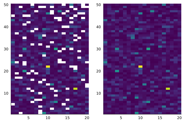

Normalization

Normalization is a process of scaling the data to a common range. This is often done to account for differences in sample concentrations. For this example, we will use the BigRiverJunbi.intnorm method, which is a simple method that normalizes the data to have a total area of 1.

# disallow missings for imputed data
imputed_data = disallowmissing(imputed_data)
# Normalize each sample (row) so total area equals 1
# This is common in metabolomics to account for dilution effects
normalized_data = BigRiverJunbi.intnorm(imputed_data; dims = 2)  # dims=2 for row-wise normalization

Transformation

Transformation is a process of transforming the data to a different distribution. For this example, we will use the BigRiverJunbi.log_tx method, which is a simple method that transforms the data to a log distribution.

# Log2 transformation with small constant to handle near-zero values
# Common in 'omics to make data more normally distributed
transformed_data = BigRiverJunbi.log_tx(normalized_data; base = 2, constant = 1e-6)

Standardization

Standardization is a process of scaling the data to have a mean of 0 and a standard deviation of 1. This is often done to account for differences in sample concentrations.

# Standardize features (columns) to have mean=0 and std=1
# Essential for many machine learning algorithms
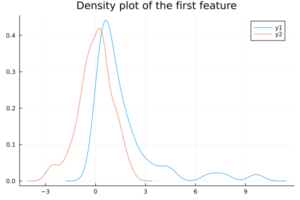
standardized_data = BigRiverJunbi.standardize(transformed_data; center = true)

We can now compare the distribution of the first feature of the data before and after the transformation:

density(imputed_data[:, 1], title="Density plot of the first feature")
density!(standardized_data[:, 1])